MPSlib: Hard and soft data
MPSlib can account for hard and soft data (both co-located and non-co-located). Details about the use of the preferential path and co- and non-co-located soft data can be found in:
mps_snesim_tree and mps_snesim_list can account for co-located soft data only.
mps_genesim can account for both co-located and non-co-located soft data.
Define hard data
Hard data (model parameters with no uncertainty) are given by the d_hard variable, with X, Y, Z, and VALUE for each conditional data point. Three conditional hard data can be given by:
O.d_hard = np.array([[ ix1, iy1, iz1, val1],
                     [ ix2, iy2, iz2, val2],
                     [ ix3, iy3, iz3, val3]])
Define soft/uncertain data
Soft data (model parameters with uncertainty) are given by the d_soft variable, with X, Y, Z for the position and a probability for each possible outcome. When considering a training image with two categories [0, 1], setting P(m=0)=0.2 at position [5, 3, 2] is done as:
O.d_soft = np.array([[ 5, 3, 2, 0.2, 0.8]])
If a training image has 3 categories and P(m=0)=0.2, P(m=1)=0.3, then:
O.d_soft = np.array([[ 5, 3, 2, 0.2, 0.3, 0.5]])
Preferential path
MPSlib supports a preferential simulation path such that model parameters with more informative conditional data (i.e. lower entropy) are simulated before less informed nodes. This is especially useful when using sparse soft data.
O.par['shuffle_simulation_grid'] = 0  # Unilateral path
O.par['shuffle_simulation_grid'] = 1  # Random path
O.par['shuffle_simulation_grid'] = 2  # Preferential path
Co-located soft data
By default, only co-located soft data are considered during simulation:
O.par['n_cond_soft'] = 1              # Only 1 soft data point is used
O.par['max_search_radius_soft'] = 0   # Only co-located soft data is used
O.par['shuffle_simulation_grid'] = 2  # Preferential path
It is advised to use the preferential path whenever using co-located soft data.
Non-co-located soft data
mps_genesim can handle non-co-located soft data using a rejection sampler. In practice, it becomes computationally expensive to condition on many soft data points. To use up to 3 soft data points within a search radius:
O.par['n_cond_soft'] = 3
O.par['max_search_radius_soft'] = 10000000
O.par['shuffle_simulation_grid'] = 2  # Preferential path
Using the preferential path is always recommended.
[1]:
import mpslib as mps
import numpy as np
import matplotlib.pyplot as plt
Setup
[2]:
#O = mps.mpslib(method='mps_snesim_tree', parameter_filename='mps_snesim.txt')
O = mps.mpslib(method='mps_genesim', parameter_filename='mps_genesim.txt')

TI1, TI_filename1 = mps.trainingimages.strebelle(3, coarse3d=1)
O.par['soft_data_categories'] = np.array([0, 1])
O.ti = TI1
Using mps_genesim installed in /mnt/space/space_au11687/PROGRAMMING/mpslib (scikit-mps in /mnt/space/space_au11687/PROGRAMMING/mpslib/scikit-mps/mpslib/mpslib.py)
[3]:
O.par['rseed'] = 1
O.par['n_multiple_grids'] = 0
O.par['n_cond'] = 16
O.par['n_cond_soft'] = 1
O.par['n_real'] = 500
O.par['debug_level'] = -1
O.par['simulation_grid_size'][0] = 18
O.par['simulation_grid_size'][1] = 13
O.par['simulation_grid_size'][2] = 1
O.par['hard_data_fnam'] = 'hard.dat'
O.par['soft_data_fnam'] = 'soft.dat'
O.delete_local_files()
O.par['n_max_cpdf_count'] = 100
Hard data
[4]:
# Set hard data
d_hard = np.array([[ 15, 4, 0, 1],
                   [ 15, 5, 0, 1]])
# Optionally use hard data
# O.d_hard = d_hard
Soft/uncertain data
[5]:
# Set soft data
d_soft = np.array([[ 2,  2, 0, 0.7,   0.3  ],
                   [ 5,  5, 0, 0.001, 0.999],
                   [10,  8, 0, 0.999, 0.001]])

O.d_soft = d_soft
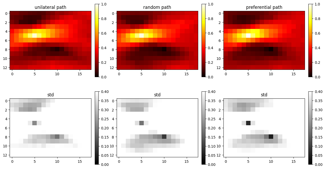
Example 1: Co-located soft data only
In this example only one soft data point is used, and only if it is located at the same position as the node being simulated in the sequential simulation.
[6]:
# Only co-located
O.par['n_cond_soft'] = 1
O.par['max_search_radius_soft'] = 0

gtxt = ['unilateral', 'random', 'preferential']
shuffle_simulation_grid_arr = [0, 1, 2]
fig = plt.figure(figsize=(15, 8))
for i in range(len(shuffle_simulation_grid_arr)):
    O.par['shuffle_simulation_grid'] = shuffle_simulation_grid_arr[i]

    O.delete_local_files()
    O.run_parallel()
    m_mean, m_std, m_mode = O.etype()

    plt.subplot(2, 3, i + 1)
    plt.imshow(m_mean.T, zorder=-1, vmin=0, vmax=1, cmap='hot')
    plt.colorbar(fraction=0.046, pad=0.04)
    plt.title('%s path' % gtxt[i])
    plt.subplot(2, 3, 3 + i + 1)
    plt.imshow(m_std.T, zorder=-1, vmin=0, vmax=0.4, cmap='gray')
    plt.title('std')
    plt.colorbar(fraction=0.046, pad=0.04)
parallel: Using 25 of max 26 threads
parallel: Using 25 of max 26 threads
parallel: Using 25 of max 26 threads
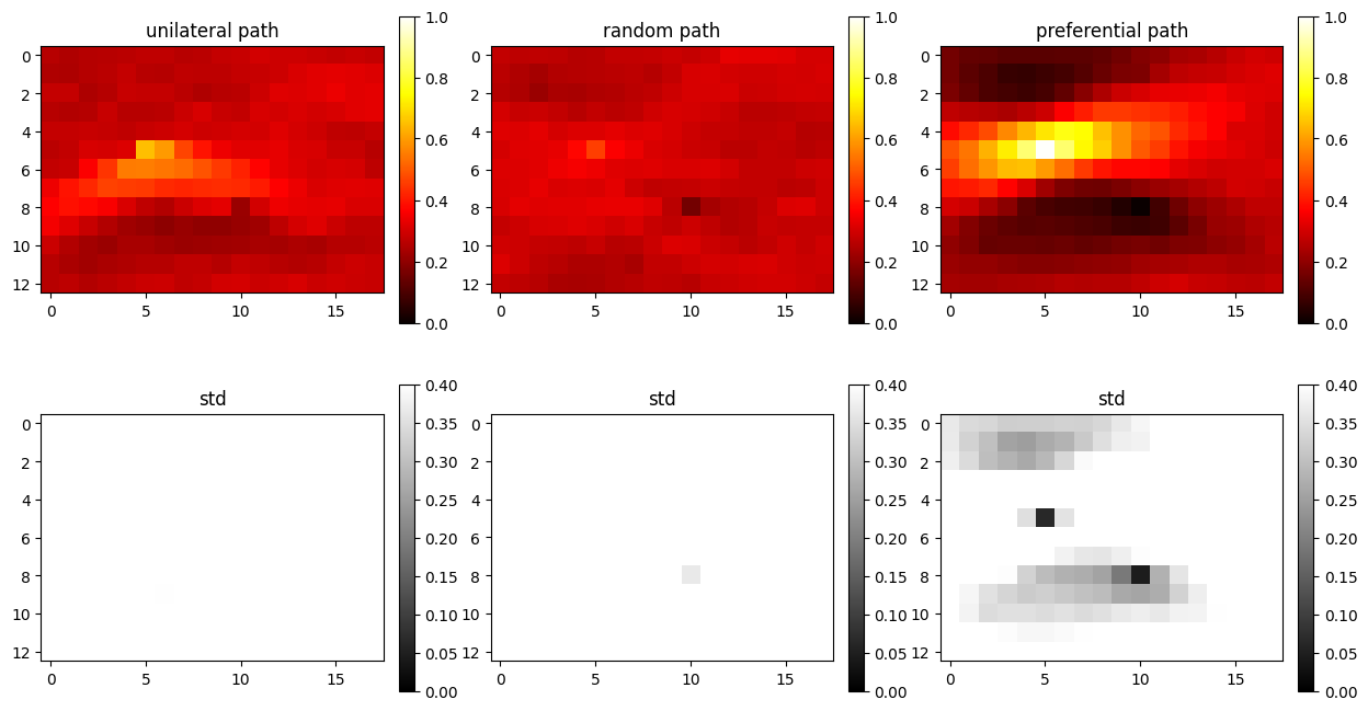
Example 2: One non-co-located soft data point
In this example still only one soft data point is used, but it can be located anywhere in the simulation grid.
[7]:
# One non-co-located soft data point
O.par['n_cond_soft'] = 1
O.par['max_search_radius_soft'] = 1000000

shuffle_simulation_grid_arr = [0, 1, 2]
fig = plt.figure(figsize=(15, 8))
for i in range(len(shuffle_simulation_grid_arr)):
    O.par['shuffle_simulation_grid'] = shuffle_simulation_grid_arr[i]

    O.delete_local_files()
    O.run_parallel()
    m_mean, m_std, m_mode = O.etype()

    plt.subplot(2, 3, i + 1)
    plt.imshow(m_mean.T, zorder=-1, vmin=0, vmax=1, cmap='hot')
    plt.colorbar(fraction=0.046, pad=0.04)
    plt.title('%s path' % gtxt[i])
    plt.subplot(2, 3, 3 + i + 1)
    plt.imshow(m_std.T, zorder=-1, vmin=0, vmax=0.4, cmap='gray')
    plt.title('std')
    plt.colorbar(fraction=0.046, pad=0.04)
parallel: Using 25 of max 26 threads
parallel: Using 25 of max 26 threads
parallel: Using 25 of max 26 threads
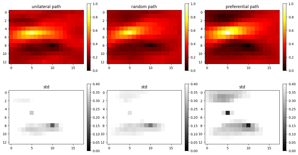
Example 3: Three (all) non-co-located soft data points
[8]:
# Three non-co-located soft data points
O.par['n_cond_soft'] = 3
O.par['max_search_radius_soft'] = 1000000

shuffle_simulation_grid_arr = [0, 1, 2]
fig = plt.figure(figsize=(15, 8))
for i in range(len(shuffle_simulation_grid_arr)):
    O.par['shuffle_simulation_grid'] = shuffle_simulation_grid_arr[i]

    O.delete_local_files()
    O.run_parallel()
    m_mean, m_std, m_mode = O.etype()

    plt.subplot(2, 3, i + 1)
    plt.imshow(m_mean.T, zorder=-1, vmin=0, vmax=1, cmap='hot')
    plt.colorbar(fraction=0.046, pad=0.04)
    plt.title('%s path' % gtxt[i])
    plt.subplot(2, 3, 3 + i + 1)
    plt.imshow(m_std.T, zorder=-1, vmin=0, vmax=0.4, cmap='gray')
    plt.title('std')
    plt.colorbar(fraction=0.046, pad=0.04)
parallel: Using 25 of max 26 threads
parallel: Using 25 of max 26 threads
parallel: Using 25 of max 26 threads