Example: Mapping buried valleys in Kasted, Denmark

import mpslib as mps
import numpy as np
import matplotlib.pyplot as plt

Get the training image and conditional data

# Get the training image
dx = 400  # Lowest resolution - faster
dx = 200
#dx = 100
#dx = 50  # Highest resolution - slower
TI, TI_fname = mps.trainingimages.kasted(dx=dx)

url_base = 'https://raw.githubusercontent.com/ergosimulation/mpslib/master/data/kasted'
remote_files = ['kasted_soft_well.dat', 'kasted_soft_ele.dat', 'kasted_soft_res.dat', 'kasted_hard_well_consistent.dat']
for local_file in remote_files:
    mps.trainingimages.get_remote('%s/%s' % (url_base, local_file), local_file)

# Get conditional point data
EAS_well = mps.eas.read(remote_files[0])
EAS_ele = mps.eas.read(remote_files[1])
EAS_res = mps.eas.read(remote_files[2])
EAS_well_hard = mps.eas.read(remote_files[3])

Set up the simulation grid geometry

# Setup the geometry
x_pad = 4 * dx
x_min = np.min(EAS_well['D'][:, 0]) - x_pad
x_max = np.max(EAS_well['D'][:, 0]) + x_pad
y_min = np.min(EAS_well['D'][:, 1]) - x_pad
y_max = np.max(EAS_well['D'][:, 1]) + x_pad
z_min = np.min(EAS_well['D'][:, 2])
z_max = np.max(EAS_well['D'][:, 2])
x_min = dx * np.floor(x_min / dx)
y_min = dx * np.floor(y_min / dx)
z_min = dx * np.floor(z_min / dx)

nx = np.int16(np.ceil((x_max - x_min) / dx))
ny = np.int16(np.ceil((y_max - y_min) / dx))
nz = np.max([np.int16(np.ceil((z_max - z_min) / dx)), 1])

grid_cell_size = np.array([1, 1, 1]) * dx
origin = np.array([x_min, y_min, z_min])
simulation_grid_size = np.array([nx, ny, nz])

print('Origin = [x0,y0,z0]=[%g,%g,%g]' % (origin[0], origin[1], origin[2]))
print('Grid cell size [dx,dy,dz]=[%g,%g,%g]' % (grid_cell_size[0], grid_cell_size[1], grid_cell_size[2]))
print('Simulation grid size [nx,ny,nz]=[%d,%d,%d]' % (simulation_grid_size[0], simulation_grid_size[1], simulation_grid_size[2]))
print('X:[%g,%g] Y:[%g,%g] Z:[%g,%g]' % (x_min, x_max, y_min, y_max, z_min, z_max))

Origin = [x0,y0,z0]=[560800,6.2246e+06,0]
Grid cell size [dx,dy,dz]=[200,200,200]
Simulation Grid size [nx,ny,nz]=[82,58,1]
X:[560800,577187] Y:[6.2246e+06,6.2362e+06] Z:[0,0]

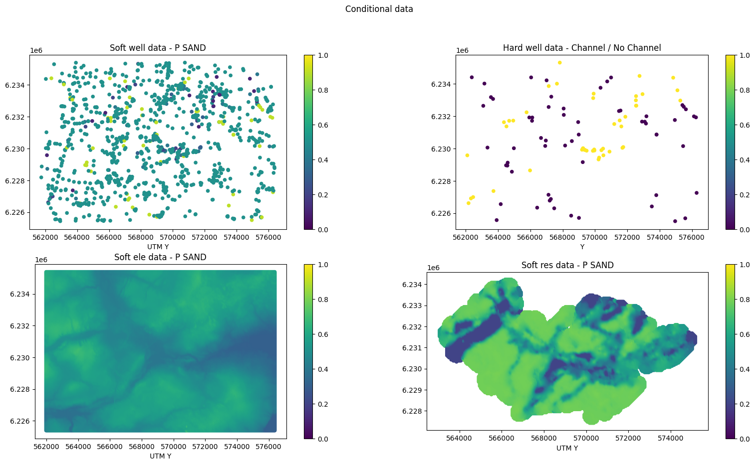
Plot the training image and the conditional data

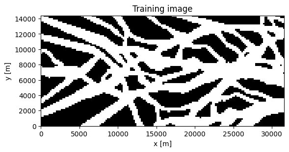
# Training image
plt.figure()
plt.imshow(TI[:, :, 0].T, cmap='gray', origin='lower', extent=[0, dx * TI.shape[0], 0, dx * TI.shape[1]])
plt.title('Training image')
plt.xlabel('x [m]')
plt.ylabel('y [m]')

# Conditional data - 2x2 overview
fig, axs = plt.subplots(2, 2, figsize=(20, 10))

# Soft well data
scatter_soft = axs[0, 0].scatter(EAS_well['D'][:, 0], EAS_well['D'][:, 1], c=EAS_well['D'][:, 3], s=20, vmin=0, vmax=1)
axs[0, 0].set_title('Soft well data - %s' % EAS_well['header'][3])
axs[0, 0].set_xlabel(EAS_well['header'][0])
axs[0, 0].set_ylabel(EAS_well['header'][1])
axs[0, 0].set_aspect('equal', 'box')
fig.colorbar(scatter_soft, ax=axs[0, 0])

# Hard well data
scatter_hard = axs[0, 1].scatter(EAS_well_hard['D'][:, 0], EAS_well_hard['D'][:, 1], c=EAS_well_hard['D'][:, 3], s=20)
axs[0, 1].set_title('Hard well data - %s' % EAS_well_hard['header'][3])
axs[0, 1].set_xlabel(EAS_well_hard['header'][0])
axs[0, 1].set_ylabel(EAS_well_hard['header'][1])
axs[0, 1].set_aspect('equal', 'box')
fig.colorbar(scatter_hard, ax=axs[0, 1])

# ELE data
scatter_ele = axs[1, 0].scatter(EAS_ele['D'][:, 0], EAS_ele['D'][:, 1], c=EAS_ele['D'][:, 3], s=20, vmin=0, vmax=1)
axs[1, 0].set_title('Soft ele data - %s' % EAS_ele['header'][3])
axs[1, 0].set_xlabel(EAS_ele['header'][0])
axs[1, 0].set_ylabel(EAS_ele['header'][1])
axs[1, 0].set_aspect('equal', 'box')
fig.colorbar(scatter_ele, ax=axs[1, 0])

# RES data
scatter = axs[1, 1].scatter(EAS_res['D'][:, 0], EAS_res['D'][:, 1], c=EAS_res['D'][:, 3], s=20, vmin=0, vmax=1)
axs[1, 1].set_title('Soft res data - %s' % EAS_res['header'][3])
axs[1, 1].set_xlabel(EAS_res['header'][0])
axs[1, 1].set_ylabel(EAS_res['header'][1])
axs[1, 1].set_aspect('equal', 'box')
fig.colorbar(scatter, ax=axs[1, 1])

fig.suptitle('Conditional data')

Text(0.5, 0.98, 'Conditional data')

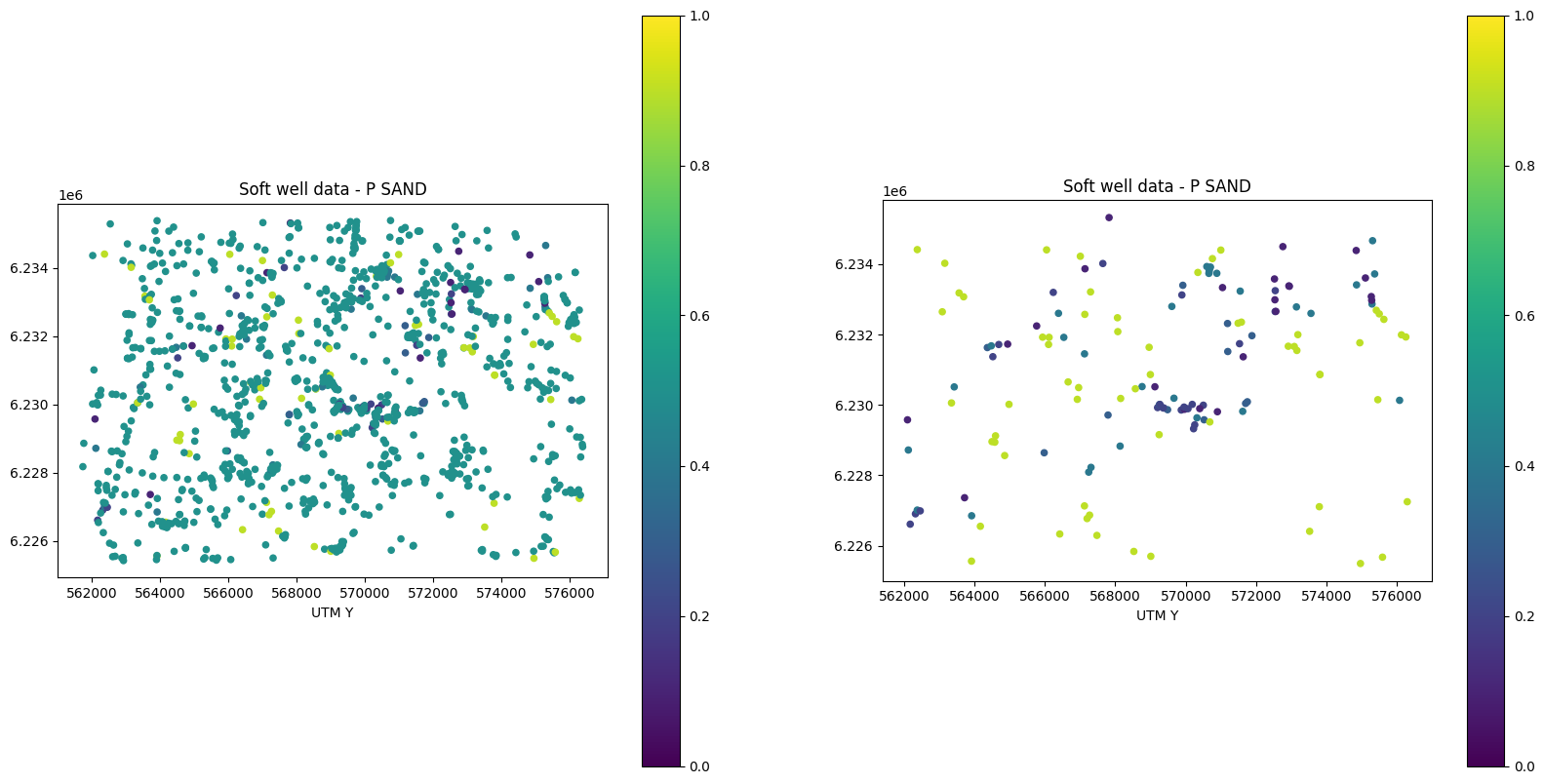
Optionally remove uninformed conditional well data

# Optionally remove non-informed conditional well data
RemoveUninformed = True

if RemoveUninformed:

    fig, axs = plt.subplots(1, 2, figsize=(20, 10))
    # Before
    scatter_soft = axs[0].scatter(EAS_well['D'][:, 0], EAS_well['D'][:, 1], c=EAS_well['D'][:, 3], s=20, vmin=0, vmax=1)
    axs[0].set_title('Soft well data - before filtering')
    axs[0].set_aspect('equal', 'box')
    fig.colorbar(scatter_soft, ax=axs[0])

    print(EAS_well['D'].shape)
    informed_well_soft_data = np.argwhere(np.abs(EAS_well['D'][:, 4] - 0.5) > 0.05)
    i_use = informed_well_soft_data.flatten()
    EAS_well['D'] = EAS_well['D'][i_use, :]
    print(EAS_well['D'].shape)

    # After
    scatter_soft = axs[1].scatter(EAS_well['D'][:, 0], EAS_well['D'][:, 1], c=EAS_well['D'][:, 3], s=20, vmin=0, vmax=1)
    axs[1].set_title('Soft well data - after filtering')
    axs[1].set_aspect('equal', 'box')
    fig.colorbar(scatter_soft, ax=axs[1])

(1254, 5)
(147, 5)

MPSlib applied to Kasted

Given the data above, the challenge is to estimate the probability that a buried valley exists in the area.

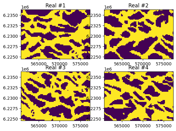
Unconditional simulation

method = 'mps_genesim'
method = 'mps_snesim_tree'
O = mps.mpslib(method=method,
               simulation_grid_size=simulation_grid_size,
               origin=origin,
               grid_cell_size=grid_cell_size)
O.par['n_real'] = 4
O.ti = TI

# Make sure to delete any local files from previous runs
O.delete_local_files()

O.run_parallel()

O.plot_reals()
#O.plot_etype()

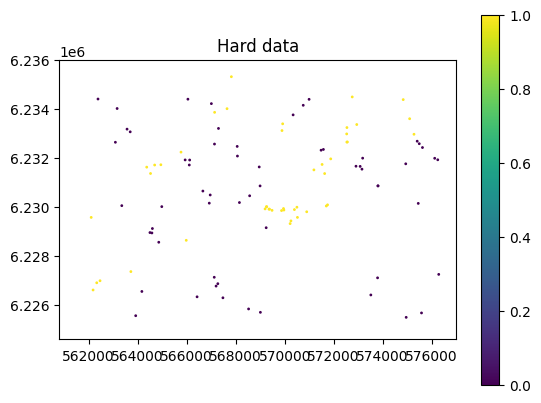
Conditional simulation - hard data

Adjust the simulation parameters to use hard conditional data. For help, see the documentation and the hard and soft data example.

method = 'mps_genesim'
#method = 'mps_snesim_tree'
O = mps.mpslib(method=method,
               simulation_grid_size=simulation_grid_size,
               origin=origin,
               grid_cell_size=grid_cell_size)
O.ti = TI

O.par['n_real'] = 50
O.par['n_cond'] = 9
O.par['n_max_ite'] = 1000
# Conditional simulation - hard data
O.d_hard = EAS_well_hard['D']
O.plot_hard()

O.run_parallel()

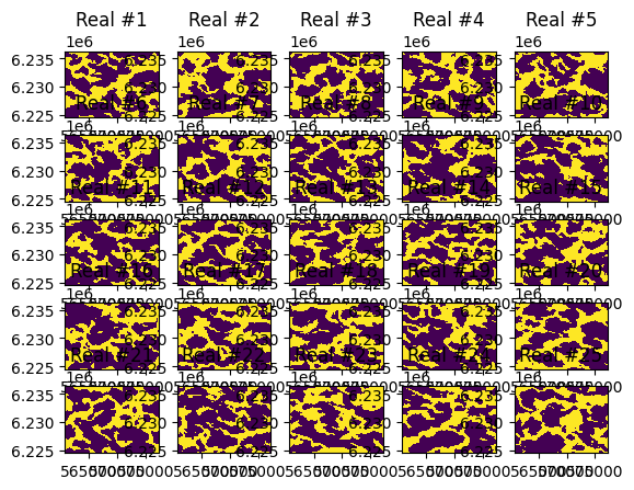
O.plot_reals()
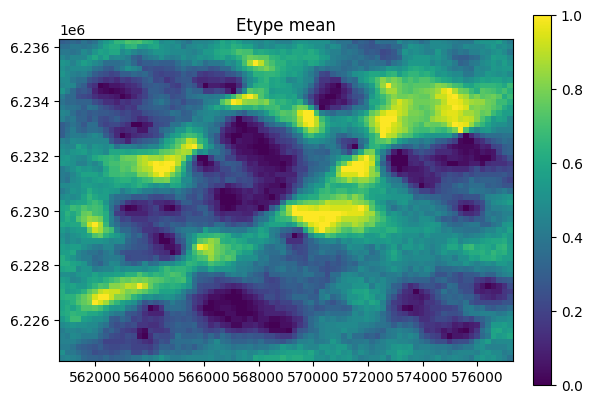
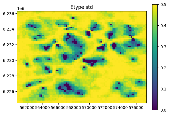
O.plot_etype()

Using mps_snesim_tree installed in /mnt/space/space_au11687/PROGRAMMING/mpslib (scikit-mps in /mnt/space/space_au11687/PROGRAMMING/mpslib/scikit-mps/mpslib/mpslib.py)
parallel: Using 4 of max 26 threads

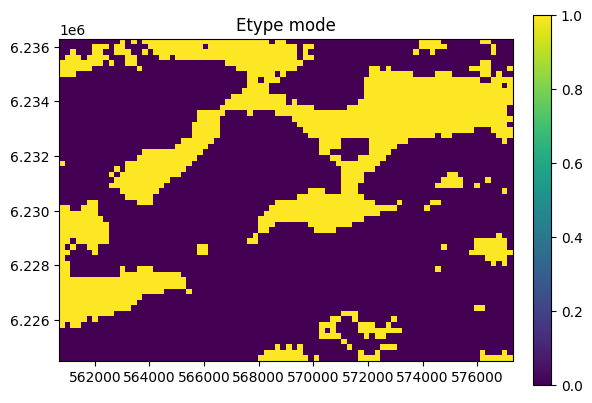
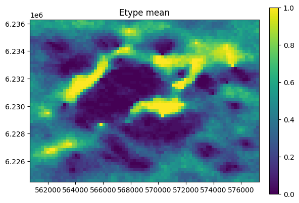
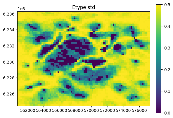
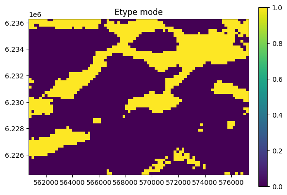
Conditional simulation - soft data

method = 'mps_genesim'
#method = 'mps_snesim_tree'
O = mps.mpslib(method=method,
               simulation_grid_size=simulation_grid_size,
               origin=origin,
               grid_cell_size=grid_cell_size)
O.delete_local_files()
O.ti = TI

O.par['n_real'] = 50
O.par['n_cond'] = 9
O.par['n_max_ite'] = 10000

O.par['n_max_cpdf_count'] = 1    # DS style
O.par['n_max_cpdf_count'] = 100  # GENESIM style

O.par['n_cond_soft'] = 1              # Only 1 soft data point is used
O.par['max_search_radius_soft'] = 0   # Only co-located soft data is used
O.par['shuffle_simulation_grid'] = 2  # Preferential path

# Select soft data
#O.d_soft = EAS_ele['D']
O.d_soft = EAS_res['D']

O.run_parallel()
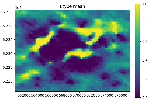
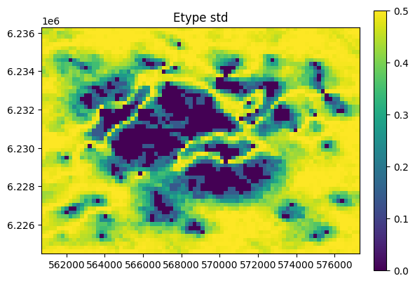
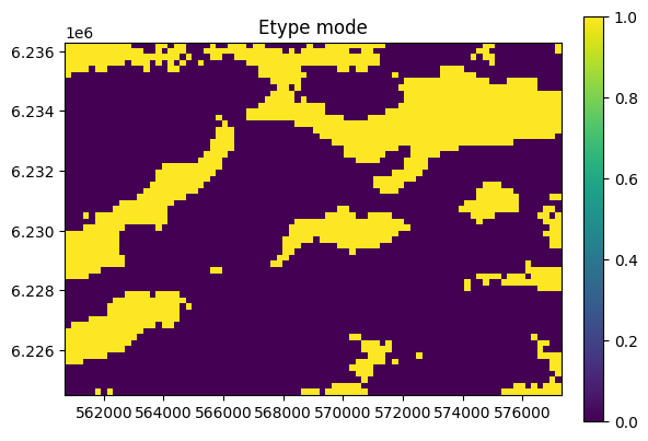
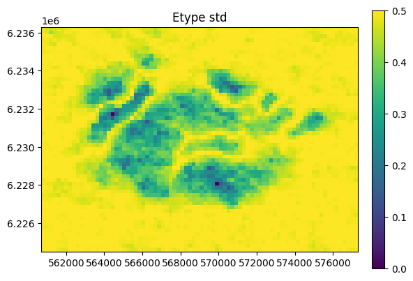
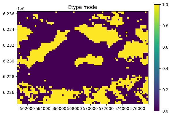
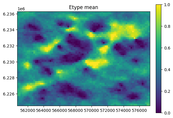
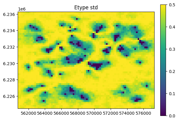
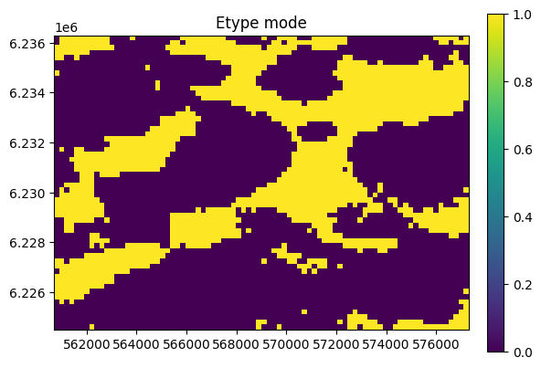
O.plot_etype()

Using mps_genesim installed in /mnt/space/space_au11687/PROGRAMMING/mpslib (scikit-mps in /mnt/space/space_au11687/PROGRAMMING/mpslib/scikit-mps/mpslib/mpslib.py)

parallel: Using 25 of max 26 threads

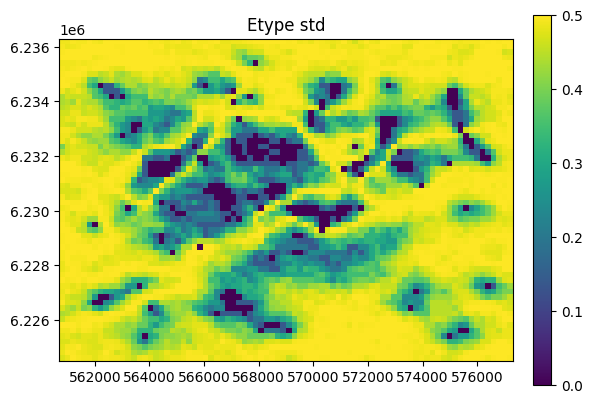
Conditional simulation - hard and soft data

method = 'mps_genesim'
#method = 'mps_snesim_tree'
O = mps.mpslib(method=method,
               simulation_grid_size=simulation_grid_size,
               origin=origin,
               grid_cell_size=grid_cell_size)
O.delete_local_files()
O.ti = TI

O.par['n_real'] = 50
O.par['n_cond'] = 9
O.par['n_max_ite'] = 10000

O.par['n_max_cpdf_count'] = 1    # DS style
O.par['n_max_cpdf_count'] = 100  # GENESIM style

O.par['n_cond_soft'] = 1                    # Only 1 soft data point is used
O.par['max_search_radius_soft'] = 1000000   # Non-co-located soft data allowed
O.par['shuffle_simulation_grid'] = 2        # Preferential path

# Select hard data
O.d_hard = EAS_well_hard['D']
O.plot_hard()

# Select soft data
O.d_soft = EAS_res['D']
O.plot_soft()

O.delete_local_files()

for n_cond_soft in [0, 1, 2, 4]:
    O.par['n_cond_soft'] = n_cond_soft

    O.run_parallel()
    print('%s: n_cond_soft=%d, %fs' % (O.method, O.par['n_cond_soft'], O.time))
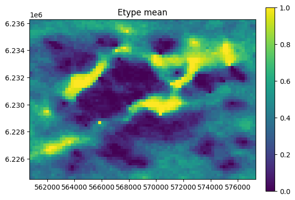
    O.plot_etype()

Using mps_genesim installed in /mnt/space/space_au11687/PROGRAMMING/mpslib (scikit-mps in /mnt/space/space_au11687/PROGRAMMING/mpslib/scikit-mps/mpslib/mpslib.py)
parallel: Using 25 of max 26 threads

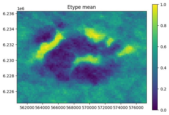
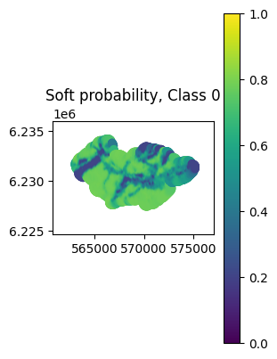
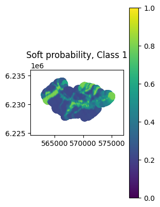
Conditional estimation - hard and soft data

Adjust the simulation parameters to perform MPS estimation instead of simulation.

O.par['do_estimation'] = 1
O.par['n_cond'] = 5
O.par['n_cond_soft'] = 4
O.run()

P0 = O.est[0][:, :, 0].T
P1 = O.est[1][:, :, 0].T
plt.imshow(P1)

Using mps_genesim installed in /mnt/space/space_au11687/PROGRAMMING/mpslib (scikit-mps in /mnt/space/space_au11687/PROGRAMMING/mpslib/scikit-mps/mpslib/mpslib.py)

parallel: Using 25 of max 26 threads
mps_genesim: n_cond_soft=0, 27.264137s

parallel: Using 25 of max 26 threads
mps_genesim: n_cond_soft=1, 26.837944s

parallel: Using 25 of max 26 threads
mps_genesim: n_cond_soft=2, 27.171099s

parallel: Using 25 of max 26 threads
mps_genesim: n_cond_soft=4, 25.545302s