scikit-mps: a Python interface to MPSlib

scikit-mps

scikit-mps [https://pypi.org/project/scikit-mps/] is a Python module that interfaces to MPSlib.

It can be installe using pip by (see details at https://pypi.org/project/scikit-mps/):

pip install scikit-mps

Or from the source code located in the mpslib/scikit-mps folder, using

cd mpslib/scikit-mps
pip install .

To allow editing scikit-mps locally after install use

cd mpslib/scikit-mps
pip install -e .

Several Python notebooks examples are located in mpslib/scikit-mps/examples whic can be browsed here: Python notebooks.

It includes 4 submodules

mps.mpslib
mps.eas
mps.trainingimages
mps.plot

and

mps.mpslib contains the core function for setting up and running the algorithms in MPSlib. mps.eas contains function to read and write EAS formatted ASCII files. mps.trainingimages provides easy access to 2D and 3D training images. mps.plot provides 2D/3D plotting utilities.

It makes use of matplotlib (for 2D graphics) and pyvista [http://docs.pyvista.org/] (for 3D graphics).

A simple example of using scikit-mps to generate 4 realizations using mps_snesim_tree is (from mpslib_simple.py):

import mpslib as mps

# Initialize the MPS object, using a specific algorithm (def='mps_snesim_tree')
O=mps.mpslib(method='mps_snesim_tree')

# Select number of realiization [def=1]
O.par['n_real']=4

# Set training image
O.ti = mps.trainingimages.strebelle()[0]
O.plot_ti()

# Run MPSlib
O.run()

# Plot the results
O.plot_reals()

O.plot_etype()

that provides Figures Fig. 5 and Fig. 6.

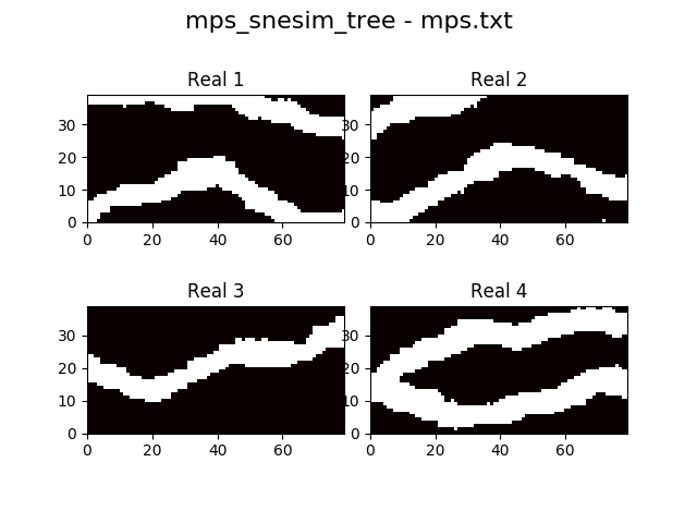
Fig. 5 Realizations from simulation

and

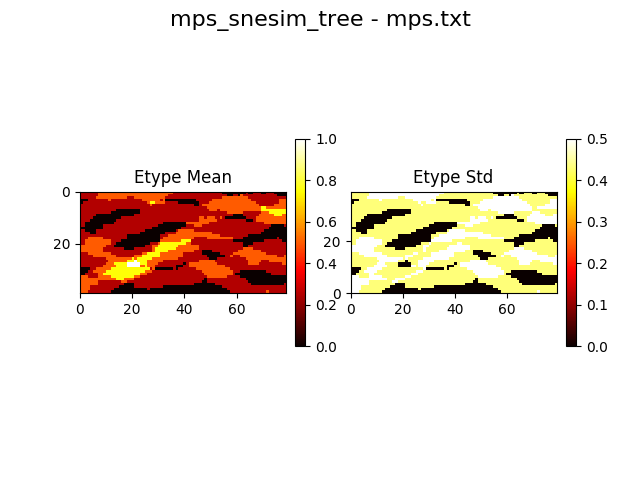
Fig. 6 Etype mean and variance from the simulation.

mps.mpslib: The main interface to MPSlib

mps.mpslib provide a class to allow running MPSlib algorithms. An instance O of the class is class can be created using:

O=mps.mpslib()

This will use a default choice of simulation method, as defined in O.method

In [1]: O.method
Out[1]: 'mps_genesim'

and a default parameter file name, as defined in O.parameter_filename

In [2]: O.parameter_filename
Out[2]: 'mps.txt'

and default parameters for the parameter file, as defined in O.par

In [3]: O.par
Out[3]:
{'n_real': 1,
'rseed': 1,
'n_max_cpdf_count': 1,
'out_folder': '.',
'ti_fnam': 'ti.dat',
'simulation_grid_size': array([80, 40,  1]),
'origin': array([0., 0., 0.]),
'grid_cell_size': array([1, 1, 1]),
'mask_fnam': 'mask.dat',
'hard_data_fnam': 'hard.dat',
'shuffle_simulation_grid': 2,
'entropyfactor_simulation_grid': 4,
'shuffle_ti_grid': 1,
'hard_data_search_radius': 1,
'soft_data_categories': array([0, 1]),
'soft_data_fnam': 'soft.dat',
'n_threads': 1,
'debug_level': -1,
'n_cond': 36,
'n_cond_soft': 0,
'n_max_ite': 1000000,
'distance_measure': 1,
'distance_min': 0,
'distance_pow': 1,
'colocate_dimension': 0,
'max_search_radius': 10000000,
'max_search_radius_soft': 10000000}

All these parameters can be set when the object is initialized. A common approach to initialized the mpslib object is to initialize it using a specific choice a simulation algorithm, simulation grid size, number of realizations, and number of conditional points. This can be done using e.g.

O = mps.mpslib(method='mps_snesim_tree',
    simulation_grid_size(80,80,1),
    n_cond = 49
    n_real = 1)

To run the MPSlib algorithms using a single thread use:

O.run()

To run the MPSlib algorithms using a multiple threads use:

O.run_parallel()

mps.eas: reading and writing EAS formatted files

mps.eas contains several functions for reading and writing EAS formatted data.

Read EAS point set

To read a point data set, use

import mpslib as mps
EAS = mps.eas.read('data.dat')

EAS['D'] contains the data values [ndata X ncolumns] as a 2D numpy array. EAS['header'] contains the header for each columns as list of strings EAS['title'] contains the title [string] for the eas file.

Write EAS point set

To write a matrix as an EAS formatted point set

import mpslib as mps
mps.eas.write(D, filename='eas.dat', title='eas title', header=[]):

D must be a 2D numpy array. filename is the EAS file name. Optionally header [list of strings] and title [string] can be set.

Read EAS volume set

An EAS volume data set, is a special version of the EAS file format that allow describing a 1D-3D volume. The first line (the title) must contain the dimensions of the data in the eas file formatted as e.g.

100 210 13

to describe a matrix of size nx=100, ny=210, and nz=13. It is read as for the points data set

import mpslib as mps
EAS = mps.eas.read('ti.dat')

EAS['Dmat'] contains a 3D numpy array of shape (100,210,13)

Write EAS volume set

A 3D numpy array can be written as an EAS volume set using

import mpslib as mps
import numpy as no
D = np.zeros((20,10,30))
mps.eas.write_mat(D,filename='D,dat')

mps.trainingimages: Easy access to training images.

mps.traningimages contain easy access to a large number of training images. To see a list of the available training images call

In [40]: mps.trainingimages.ti_list()
Available training images:
checkerboard - 2D checkerboard
checkerboard2 - 2D checkerboard - alternative
strebelle - 2D discrete channels from Strebelle
lines - 2D discrete lines
stones - 2D continious stones
bangladesh - 2D discrete Bangladesh
maze - 2D discrete maze
rot90 - 3D rotation 90
rot20 - 3D rotation 20
horizons - 3D continious horizons
fluvsim - 3D discrete fluvsim

To load and plot the widely used training image from Strebelle, simply call it using e.g.

import mpslib as mps
ti, ti_filename = mps.trainingimages.strebelle()
mps.plot.plot_3d(ti)

To load and plot a checkerboard training image, use e.g

import mpslib as mps
ti, ti_filename = mps.trainingimages.checkerboard()
mps.plot.plot_3d(ti)

To load and plot the 3D fluvsim training image, use e.g

import mpslib as mps
ti, ti_filename = mps.trainingimages.fluvsim()
mps.plot.plot_3d(ti)

mps.plot: Plotting utilities

‘’mps.plot’’ contains a number of functions for plotting mpslib data and realizations in 2D (using matplotlib) and 3D (using pyvista).

plot_reals_3d()

To plot several realizations using pyvista from a mpslib object, use

import mpslib as mps
O = mps.mpslib(n_real=4)
O.run
O.plot.plot_reals_3d(O)

To plot a 3D numpy array using pyvista use

import mpslib as mps
ti, ti_filename = mps.trainingimages.checkerboard()
mps.plot.plot_3d(ti)

To slice the 3D grid use

import mpslib as mps
ti, ti_filename = mps.trainingimages.checkerboard()
mps.plot.plot_3d(ti, slice=1)

To plot only vaĺues in a specific range, e.g. -.5 to 0.5, use

import mpslib as mps
ti, ti_filename = mps.trainingimages.checkerboard()
mps.plot.plot_3d(ti, threshold = (-0.5, 0.5))