MPSlib: Computation of entropy and self-information

The self-information, and entropy (the average self-information), can be computed using MPSlib by setting

do_entropy = 1

This works for all algorithms except when using mps_genesim in direct sampling mode (i.e. when O.par['n_max_cpdf_count'] = 1).

See details in:

Hansen, Thomas Mejer. “Entropy and information content of geostatistical models.” Mathematical Geosciences 53.1 (2021): 163-184

import numpy as np
import matplotlib.pyplot as plt
import mpslib as mps

Setup MPSlib

Setup MPSlib and select to compute entropy.

# Initialize MPSlib using the mps_snesim_tree algorithm and a simulation grid of size [80, 70, 1]
#O = mps.mpslib(method='mps_genesim', simulation_grid_size=[80, 70, 1], n_max_cpdf_count=30, verbose_level=-1)
O = mps.mpslib(method='mps_snesim_tree', simulation_grid_size=[80, 70, 1], verbose_level=-1)
O.delete_local_files()
O.par['n_real'] = 1000
O.par['n_cond'] = 9
# Choose to compute entropy
O.par['do_entropy'] = 1
TI, TI_filename = mps.trainingimages.strebelle(di=4, coarse3d=1)
O.ti = TI

O_all = O.run_parallel()

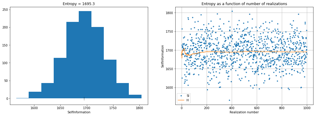
Plot entropy

fig = plt.figure(figsize=(18, 6))

plt.subplot(1, 2, 1)
plt.hist(O.SI)
plt.plot(np.array([1, 1]) * O.H, [-5, 5], 'k:')
plt.xlabel('Self-information')
plt.title('Entropy = %3.1f' % (O.H))

plt.subplot(1, 2, 2)
plt.plot(O.SI, '.', label='SI')
plt.plot(np.cumsum(O.SI) / (np.arange(1, 1 + len(O.SI))), '-', label='H')
plt.legend()
plt.grid()
plt.xlabel('Realization number')
plt.ylabel('Self-information')
plt.title('Entropy as a function of number of realizations')

Text(0.5, 1.0, 'Entropy as a function of number of realizations')

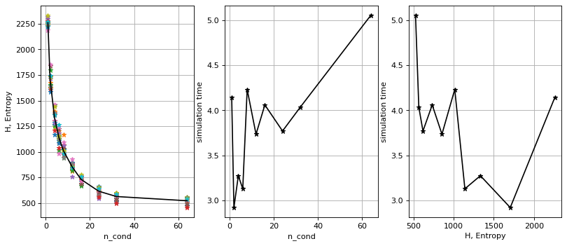
Entropy as a function of number of conditional data

TI, TI_filename = mps.trainingimages.strebelle(di=4, coarse3d=1)

n_cond_arr = np.array([1, 2, 4, 6, 8, 12, 16, 24, 32, 64])

H = np.zeros(n_cond_arr.size)  # entropy
t = np.zeros(n_cond_arr.size)  # simulation time
i = 0
SI = []
for n_cond in n_cond_arr:
    O = mps.mpslib(method='mps_snesim_tree', simulation_grid_size=[80, 70, 1], verbose_level=-1)
    O.par['n_real'] = 20
    O.par['n_cond'] = n_cond
    # Choose to compute entropy
    O.par['do_entropy'] = 1
    O.ti = TI

    O.run_parallel()
    print('n_cond = %d, H=%4.1f' % (n_cond, O.H))
    SI.append(O.SI)  # Self-information
    H[i] = O.H       # Entropy
    t[i] = O.time
    i = i + 1

n_cond = 1, H=2260.7
n_cond = 2, H=1705.0
n_cond = 4, H=1332.4
n_cond = 6, H=1138.6
n_cond = 8, H=1012.2
n_cond = 12, H=852.4
n_cond = 16, H=730.9
n_cond = 24, H=615.3
n_cond = 32, H=563.6
n_cond = 64, H=522.3

plt.figure(figsize=(12, 5), dpi=80)

ax1 = plt.subplot(1, 3, 1)
plt.plot(n_cond_arr, SI, '*')
plt.plot(n_cond_arr, H, 'k-')
plt.grid()
plt.xlabel('n_cond')
plt.ylabel('H, Entropy')

ax2 = plt.subplot(1, 3, 2)
plt.plot(n_cond_arr, t, 'k-*')
plt.grid()
plt.xlabel('n_cond')
plt.ylabel('Simulation time (s)')

ax3 = plt.subplot(1, 3, 3)
plt.plot(H, t, 'k-*')
plt.grid()
plt.xlabel('H, Entropy')
plt.ylabel('Simulation time (s)')

Text(0, 0.5, 'simulation time')