Ex: Soft/uncertain data

MPSlib can take ‘soft’ data into account. ‘soft’ data is defined as uncertain and spatially independent information about one ore more model parameters. Formally the soft information is quantified by \(f_{soft}(\mathbf{m})\) as

(1)\[\begin{split}f_{soft}(\mathbf{m}) & \sim f_{soft}(m_1, m_2, m_3, ..., m_M)\\ & = f_{soft}(m_1) \ f_{soft}(m_2) \ ... \ f_{soft}(m_M)\\ & = \prod_i^{M} f_{soft}(m_i)\end{split}\]

The assumption of spatial independence is critical. If the uncertain information is in fact spatially dependent (as is typically the case using soft data derived from inversion of geophysical data), the variability in the generated realizations will be too small, such the apparent information content is too high.

MPSlib allow conditioning to both co-located soft data (mps_snesim_tree and mps_genesim) and non-co-located soft data (mps_genesim). The implementation of soft in MPSlib is described in detail in in [HANSEN2018].

Soft data must be provided as an EAS file. If a training image with Ncat categories is used then the EAS file must contain N=3+`Ncat` columns. The first three must be ´X´, Y, and Z. The the following columns provide the probability of each category. Column 4 (the first column with soft data) refer to the probability of the category with the lowest number in the training image.

An example of defining 3 soft data, for a case with Ncat=2, and with soft information close to hard information (almost no uncertainty) is

SOFT data mimicking hard data
5
X
Y
Z
P(cat=0)
P(cat=1)
        6          14           0       0.001       0.999
        13         16           0       0.001       0.999
        3          14           0       0.999       0.001

Co-located soft data

The usual approach to handling soft data, is to conisder on co-located soft data during sequential simulation. This means that at each iteration of sequential simulation one sample from

\[f(m_i | I_{hard}, I_{soft}) = f_{TI}(m_i | \mathbf{m}_c) * f_{soft}(m_i)\]

As demonstrated in [HANSEN2018] the use of a unilateral or random path using co-located soft data leads to ignoring most of the soft information. The problem is most severe when using scattered soft data. If in stead a simulation path is chosen where more informed nodes (where the entropy of the soft data i high) are visited preferentially to less informed nodes, then much more of the soft data is being taken into account.

The default path in MPSlib is therefore the preferential path, that can selected as the path type 2 in the parameter file. The second parameter controls the randomness of the preferential path.

...
Training image file (spaces not allowed) # ti.dat
Output folder (spaces in name not allowed) # .
Shuffle Simulation Grid path (2: preferential, 1: random, 0: sequential, 2: preferential) # 2 4
Shuffle Training Image path (1 : random, 0 : sequential) # 1
...

The behavior of mps_genesim with soft data is controlled by the number of soft conditional data, and the max search radius of conditional soft data. To use co-located soft data, the number of soft data is set to 1, and the search radius is set to 0 as :

...
Max number of conditional point: Nhard, Nsoft# 16 1
...
Max Search Radius for conditional data [hard,soft] # 10000000 0
...

Figure Fig. 3 shows the point wise mean of 100 realizations using the soft data described above, in case using a sequential, random and preferential simulation path (from mpslib_hard_as_soft_data.py): .

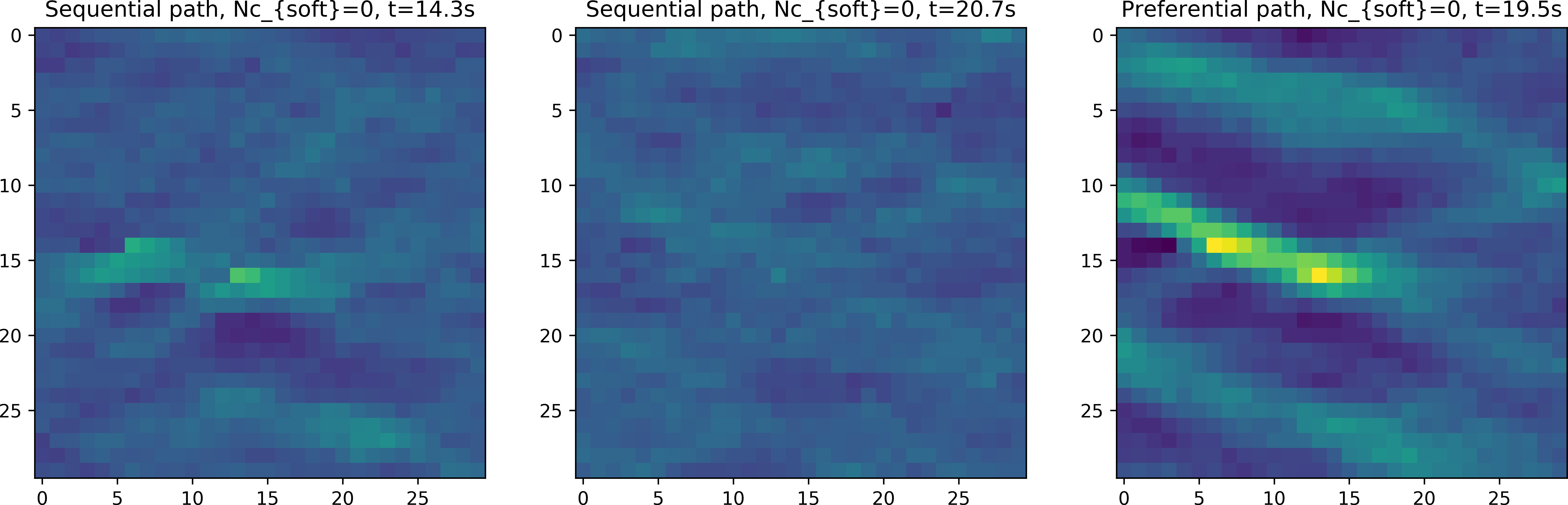
Fig. 3 E-type mean using a sequential, random and preferential simulation path, conditioning co-located soft data.

and

Non Co-located soft data

If soft information is scattered, and located relatively far away from each other, then using only co-located soft data my work well. But, when soft information is more densely available, using only co-located soft data results in disregarding available information.

mps_genesim can handle non-colocated soft information running both in ENESIM mode and Direct Sampling mode (using only 1 match in the training image). In both cases one samples from the following conditional distribution during sequential simulation:

\[f(m_i | I_{hard}, I_{soft}) = f_{TI}(m_i | \mathbf{m}_c) * \prod_{j=1}^{Nc_{soft}} f_{soft}(m_j)\]

where \(Nc_{soft}\) refer to the number of (the closest) soft conditional points to use. This number of defined right next to the maximum number of hard data used for condisioning. In order to use non-co-located soft data, the search radius for soft data must be set to a value larger than 0. In the example below, the closest 25 hard and 3 soft data is used:

:linenos:
:lineno-start: 1
:emphasize-lines: 4

Number of realizations # 1
Random Seed (0 `random` seed) # 1
Maximum number of counts for conditional pdf # 1
Max number of conditional point: Nhard, Nsoft# 25 3
Max number of iterations # 1000000
...
Max Search Radius for conditional data [hard,soft] # 10000000 10000000
...

Figure Fig. 4 shows the point wise mean of 100 realizations using a sequential, random and preferential simulation path (from mpslib_hard_as_soft_data.py) using two non-colocated soft data.

Note how the sequential and random path can in principle be used, as part of the soft data is used at each iteration, but that the simulation time is dramatically higher than using the preferential path (10 to 20 times faster). The speed is us due to the simulation of the nodes of the soft data the start of the simulation. When the soft data has been simulated, the will in effect be treated as previously simulated hard data, and hence the simulation will perform as normal conditional sequential simulation.

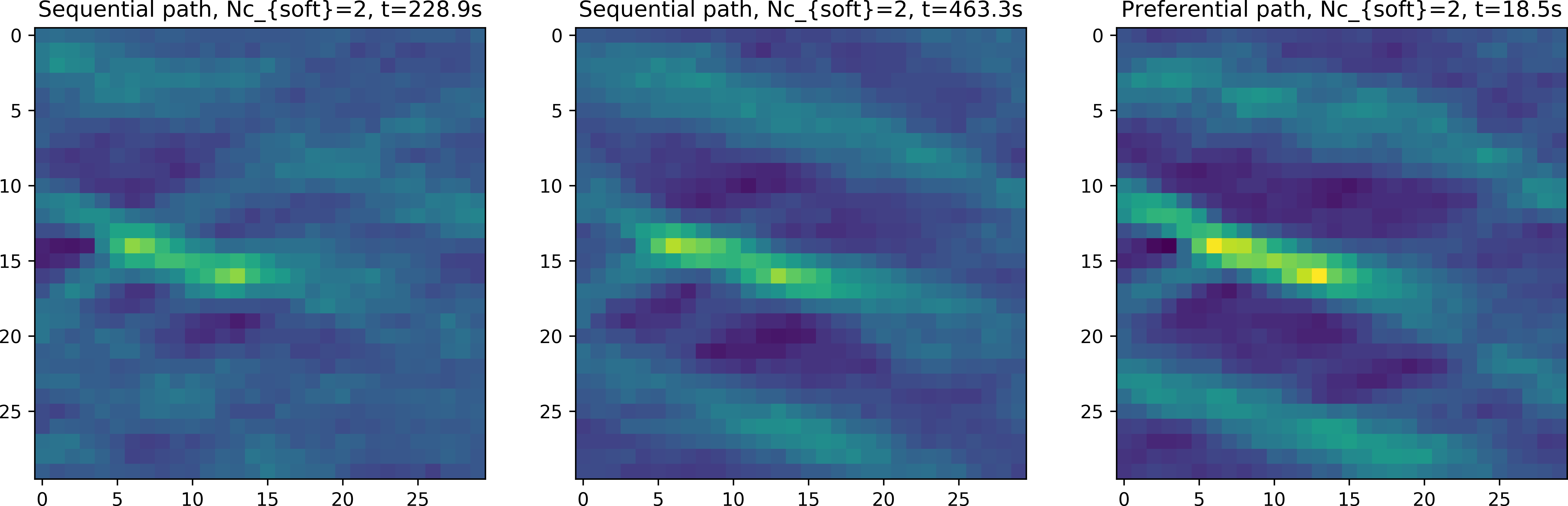
Fig. 4 E-type mean using a sequential, random and preferential simulation path, conditioning to 3 non-co-located soft data.