MPSlib: hard and soft data in MPSlib

MPSlib can account for hard and soft data (both colocated and no-colocated). Detail about the use of the preferential path and co- and non-co-located soft data can be found in

Hansen, Thomas Mejer, Klaus Mosegaard, and Knud Skou Cordua. “Multiple point statistical simulation using uncertain (soft) conditional data.” Computers & geosciences 114 (2018): 1-10

Define hard data

Hard data (model parameyers with no uncertainty) are given by the ‘’’d_hard’’’ variable, with X, Y, Z, and VALUE for each conditonal data. 3 conditional hard data can be given by

O.d_hard = np.array(  [[ ix1, iy1, iz1, val1],
                       [ ix2, iy2, iz2, val2],
                       [ ix3, iy3, iz3, val3]])

Define soft/uncertain data

Soft data (model parametrs wth no uncertainty) are given by the ‘’’d_soft variable, with X, Y, Z, for the position, and a probability of each possible outcome. When considering a training with two categories [0,1], then with P(m=0)=0.2, at position [5,3,2] can be set as

O.d_soft = np.array(  [[ 5, 3, 2, 0.2 0.8]])

If a training image has 3 categories and P(m=0)=0.2, and P(m=1)=0.3, then

O.d_soft = np.array(  [[ 5, 3, 2, 0.2, 0.4, 0.5]])

Preferential path

MPSlib makes use of a preferential simulation path, such that model parameters with more informed conditional information (i.e. wigh lower entropy) prior to less nodes with less informed conditonal information. Especially when using spare soft data, the use of a preferential path should be preferred

O.par['shuffle_simulation_grid']=0 # Unilateral path
O.par['shuffle_simulation_grid']=1 # Random path
O.par['shuffle_simulation_grid']=0 # Preferential path

co-located soft data

By default only co-located soft data are considered during simulation, as given by

O.par['n_cond_soft']=0
O.par['shuffle_simulation_grid']=0 # Preferential path

Whenever using only co-locate soft data is is adviced to use the preferential path

non-co-located soft data.

Even when using the preferential path, model parameters with informed conditional indformation, close to the point being simulated, will not be taken into account. This means in practice that not all information in soft conditional data is used. As an alternative ‘mps_genesim’ can handle non-colocated soft data, by using a rejection sample to accept a proposed match m* from scannining the TI, with a probability proprtional to the product of the condtional information evalauted in m*.

This means that one can account for, in principle, any number of soft data, as one can account for any number of hard data. In practice, it becomes computationally har to account for many soft data. To set the number of soft data used for conditining to 3, on can use

O.par['n_cond_soft']=3

When using multiple (or all) conditional soft data, then use of the preferential path may not lead to more informed realizations than using a random path, but simulation mey be sginificantly faster using the preferential path as model parameters with soft data will be simulated first, and the subsequenty simulation will be conditional to only hard data, and hence computationally more efficient. Therefore it is advised to use a preferential path always.

import mpslib as mps
import numpy as np
import matplotlib.pyplot as plt

O=mps.mpslib(method='mps_snesim_tree', parameter_filename='mps_snesim.txt')
#O=mps.mpslib(method='mps_genesim', parameter_filename='mps_genesim.txt')


TI1, TI_filename1 = mps.trainingimages.strebelle(3, coarse3d=1)
O.par['soft_data_categories']=np.array([0,1])
O.ti=TI1

#%% Set parameters for MPSlib
O.par['rseed']=1
O.par['n_multiple_grids']=0;
O.par['n_cond']=16
O.par['n_cond_soft']=1
O.par['n_real']=100
O.par['debug_level']=-1
O.par['simulation_grid_size'][0]=18
O.par['simulation_grid_size'][1]=13
O.par['simulation_grid_size'][2]=1
O.par['hard_data_fnam']='hard.dat'
O.par['soft_data_fnam']='soft.dat'
O.delete_local_files()

O.par['n_max_cpdf_count']=100

Hard data

# Set hard data
d_hard = np.array([[ 15, 4, 0, 1],
                   [ 15, 5, 0, 1]])

#O.d_hard = d_hard

Soft/uncertain data

# Set soft data
d_soft = np.array([[ 2, 2, 0, 0.7, 0.3],
                   [ 5, 5, 0, 0.001, 0.999],
                   [ 10, 8, 0, 0.999, 0.001]])

O.d_soft = d_soft

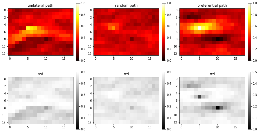
Example 1: co-locational soft data only

# Only co-locational
O.par['n_cond_soft']=0

gtxt=['unilateral','random','preferential']
shuffle_simulation_grid_arr = [0,1,2]
fig = plt.figure(figsize=(15, 8))
for i in range(len(shuffle_simulation_grid_arr)):
    # Set preferential path
    O.par['shuffle_simulation_grid']=shuffle_simulation_grid_arr[i]

    O.delete_local_files()
    O.run_parallel()
    m_mean, m_std, m_mode=O.etype()

    plt.subplot(2,3,i+1)
    plt.imshow(m_mean.T, zorder=-1, vmin=0, vmax=1, cmap='hot')
    plt.colorbar(fraction=0.046, pad=0.04)
    plt.title('%s path' % gtxt[i])
    plt.subplot(2,3,3+i+1)
    plt.imshow(m_std.T, zorder=-1, vmin=0, vmax=0.4, cmap='gray')
    plt.title('std')
    plt.colorbar(fraction=0.046, pad=0.04)

parallel: Using 10 of max 10 threads
parallel: Using 10 of max 10 threads
parallel: Using 10 of max 10 threads

Example 2: 1 non-co-locational soft data only

# Only co-locational
O.par['n_cond_soft']=1

shuffle_simulation_grid_arr = [0,1,2]
fig = plt.figure(figsize=(15, 8))
for i in range(len(shuffle_simulation_grid_arr)):
    # Set preferential path
    O.par['shuffle_simulation_grid']=shuffle_simulation_grid_arr[i]

    O.delete_local_files()
    O.run_parallel()
    m_mean, m_std, m_mode=O.etype()

    plt.subplot(2,3,i+1)
    plt.imshow(m_mean.T, zorder=-1, vmin=0, vmax=1, cmap='hot')
    plt.colorbar(fraction=0.046, pad=0.04)
    plt.title('%s path' % gtxt[i])
    plt.subplot(2,3,3+i+1)
    plt.imshow(m_std.T, zorder=-1, vmin=0, vmax=0.4, cmap='gray')
    plt.title('std')
    plt.colorbar(fraction=0.046, pad=0.04)

parallel: Using 10 of max 10 threads
parallel: Using 10 of max 10 threads
parallel: Using 10 of max 10 threads

Example 3: 3 (all) non-co-locational soft data only

# Only co-locational
O.par['n_cond_soft']=3

shuffle_simulation_grid_arr = [0,1,2]
fig = plt.figure(figsize=(15, 8))
for i in range(len(shuffle_simulation_grid_arr)):
    # Set preferential path
    O.par['shuffle_simulation_grid']=shuffle_simulation_grid_arr[i]

    O.delete_local_files()
    O.run_parallel()
    m_mean, m_std, m_mode=O.etype()

    plt.subplot(2,3,i+1)
    plt.imshow(m_mean.T, zorder=-1, vmin=0, vmax=1, cmap='hot')
    plt.colorbar(fraction=0.046, pad=0.04)
    plt.title('%s path' % gtxt[i])
    plt.subplot(2,3,3+i+1)
    plt.imshow(m_std.T, zorder=-1, vmin=0, vmax=0.4, cmap='gray')
    plt.title('std')
    plt.colorbar(fraction=0.046, pad=0.04)

parallel: Using 10 of max 10 threads
parallel: Using 10 of max 10 threads
parallel: Using 10 of max 10 threads